I was invited to judge the cybersecurity category of a hackathon recently. As a judge, I was able to see submissions and judging for all categories, and I saw a dubious choice from the quantum category judges.
In the interest of not being an asshole, I won't be discussing any details of the submission in question beyond relevant parts.
The submission used a hybrid quantum-classical deep learning model to analyze data for a particular task.
import numpy as np

import torch
from torch.autograd import Function
import torch.nn as nn

import qiskit
from qiskit import transpile
from qiskit_aer import AerSimulator

class QuantumHybridModel(nn.Module):
    def __init__(self, qubits, shots, shift=np.pi / 2):
        super().__init__()

        self.backend = AerSimulator(method="density_matrix", device="CPU")
        self.fcs = nn.Sequential(
            nn.Linear(3, 512),
            nn.ReLU(),
            nn.Linear(512, 512),
            nn.ReLU(),
            nn.Linear(512, 1024),
            nn.ReLU(),
            nn.Linear(1024, 1024),
            nn.ReLU(),
            nn.Linear(1024, 512),
            nn.ReLU(),
            nn.Linear(512, 256),
            nn.ReLU(),
            nn.Linear(256, 64),
            nn.ReLU(),
            nn.Linear(64, 2),
        )
        self.softmax = nn.Softmax(dim=-1)
        self.quantum = QuantumLayer(qubits, self.backend, shots, shift)

    def forward(self, x):
        x = self.fcs(x)
        x = self.quantum(x)
        x = self.softmax(x)
        return x

class HybridFunction(Function):
    @staticmethod
    def forward(ctx, x, quantum_circuit, shift):
        ctx.shift = shift
        ctx.quantum_circuit = quantum_circuit

        expectation_z = ctx.quantum_circuit.run(x[0].tolist())
        result = torch.tensor(expectation_z)
        ctx.save_for_backward(x)

        return result

    @staticmethod
    def backward(ctx, grad_output):
        x, = ctx.saved_tensors
        input_list = np.array(x.tolist())

        shift_right = input_list + np.ones(input_list.shape) * ctx.shift
        shift_left = input_list - np.ones(input_list.shape) * ctx.shift

        gradients = []
        for i in range(len(input_list)):
            expectation_right = ctx.quantum_circuit.run(shift_right[i])
            expectation_left = ctx.quantum_circuit.run(shift_left[i])

            gradient = torch.tensor([expectation_right]) - torch.tensor([expectation_left])
            gradients.append(gradient)
        gradients = np.array([gradients]).T
        return torch.tensor([gradients]).float() * grad_output.float(), None, None

class QuantumCircuit:
    def __init__(self, n_qubits, backend, shots):
        self._circuit = qiskit.QuantumCircuit(n_qubits)

        all_qubits = [i for i in range(n_qubits)]
        self.thetas = [qiskit.circuit.Parameter(f"theta{i}") for i in range(n_qubits)]

        self._circuit.h(all_qubits)
        self._circuit.barrier()
        for i in range(n_qubits):
            self._circuit.ry(self.thetas[i], i)

        self._circuit.measure_all()

        self.backend = backend
        self.shots = shots

    def run(self, thetas):
        t_qc = transpile(self._circuit, self.backend)
        job = self.backend.run(
            t_qc,
            parameter_binds=[{self.thetas[i]: [thetas[i]] for i in range(len(thetas))}],
            shots=self.shots
        )
        result = job.result().get_counts()

        counts = np.array(list(result.values()))
        states = list(result.keys())

        expectation = np.zeros(len(thetas))
        for qubit in range(len(thetas)):
            prob = sum(counts[i] for i, s in enumerate(states) if s[-(qubit + 1)] == '1') / self.shots
            expectation[qubit] = prob

        return np.array([expectation])

class QuantumLayer(nn.Module):
    def __init__(self, qubits, backend, shots, shift):
        super(QuantumLayer, self).__init__()
        self.quantum_circuit = QuantumCircuit(qubits, backend, shots)
        self.shift = shift

    def forward(self, x):
        return HybridFunction.apply(x, self.quantum_circuit, self.shift)

m = QuantumHybridModel(2, 1000)
There's obviously a lot to unpack here.
At the most basic level, we have this QuantumHybridModel class which acts as our neural network module. The forward propagation for this model first performs a series of fully-connected layers with ReLU activations, starting from 3 inputs and ending with 2 outputs. Afterwards, the quantum portion comes in, taking the 2 outputs from the fully-connected layers, doing some calculations on them, and returning 2 outputs. And the final step is a simple softmax.
Seems harmless right? Perhaps a little odd to stick the quantum layer in there, but surely it's doing something valuable... Right...?
Unfortunately not. The authors justified this quantum layer by claiming it allows them to represent more states with fewer model parameters, saving memory and computational cost. This is a very funny claim to me and you'll see why very soon.
There's a bit of process to defining a custom layer in PyTorch, which is why this code sample is a little long. In order to get proper backpropagation on a non-differentiable computation, we need to subclass the torch.autograd.Function class and define our forward() and backward() functions manually. Then in the actual QuantumLayer class, we just apply our custom HybridFunction in the forward() method.
So let's start figuring out what this layer actually computes. For the forward propagation, we appear to simply be calling our QuantumCircuit run() method on the input. So what does this do?
To understand, we first need to see what happens in the QuantumCircuit constructor.
def __init__(self, n_qubits, backend, shots):
    self._circuit = qiskit.QuantumCircuit(n_qubits)

    all_qubits = [i for i in range(n_qubits)]
    self.thetas = [qiskit.circuit.Parameter(f"theta{i}") for i in range(n_qubits)]

    self._circuit.h(all_qubits)
    for i in range(n_qubits):
        self._circuit.ry(self.thetas[i], i)

    self._circuit.measure_all()

    self.backend = backend
    self.shots = shots
We define a Qiskit quantum circuit with some number of qubits, which in this case is 2. We then define a circuit parameter for each qubit, which is a way of using an arbitrary value as a quantum gate parameter. And then we get into the actual quantum computation.
The circuit first performs a Hadamard gate on all qubits. For those unfamiliar with quantum computing, this essentially puts qubits into an equal superposition of the two quantum basis states \(|0\rangle\) and \(|1\rangle\). Put simply, the qubits now "hold both values at the same time."
After the Hadamard gate, the circuit performs an Ry gate on each qubit, using the corresponding theta parameter as the angle parameter. An Ry gate takes a quantum state and rotates it around the Bloch sphere about the y-axis by the angle parameter. And for those unfamiliar with the Bloch sphere, it is essentially a representation of the possible states a qubit can hold, which is far more than the 2 you get with a classical bit.
After this we just measure the states of the qubits, which collapses them to \(|0\rangle\) or \(|1\rangle\).
So what is wrong with this, you might ask. It's definitely doing something, right? To answer this question, we need to dive a little deeper into the math behind these gates.
The Hadamard gate operator can be represented as the following linear operator:
$$ H=\frac{1}{\sqrt{2}} \begin{pmatrix} 1 & 1 \\ 1 & -1 \end{pmatrix} $$
The qubits start at the \(|0\rangle\) state, which as a vector is \(\begin{bmatrix}1 \\ 0\end{bmatrix}\), and thus after the Hadamard gate is applied, we obtain \(\frac{1}{\sqrt{2}}\begin{bmatrix}1 \\ 1\end{bmatrix}\), or \(\frac{1}{\sqrt{2}}(|0\rangle + |1\rangle)\) as the Dirac vector notation is actually a representation of a linear combination of the two basis states.
Now we move on to the Ry gate, which as a linear operator has this representation:
$$ R_y(\theta)=\begin{pmatrix}\cos(\theta/2)&-\sin(\theta/2) \\ \sin(\theta/2)&\cos(\theta/2)\end{pmatrix} $$
Seems like our state representation is gonna get a little complicated, but don't worry it'll simplify in a bit. After applying this operator, we get that our qubit has state \(\frac{1}{\sqrt{2}}((\cos(\theta/2)-\sin(\theta/2))|0\rangle+(\cos(\theta/2)+\sin(\theta/2))|1\rangle)\), or as a vector, \(\frac{1}{\sqrt{2}}\begin{bmatrix}\cos(\theta/2)-\sin(\theta/2) \\ \cos(\theta/2)+\sin(\theta/2)\end{bmatrix}\).
Thankfully, now all we do is measure. The probability of the qubit collapsing to a given basis state is just the square of the corresponding coefficient in the state vector, so the probability that we collapse to \(|1\rangle\) is \((\frac{1}{\sqrt{2}}(\cos(\theta/2)+\sin(\theta/2)))^2=\frac{1}{2}(\cos^2(\theta/2)+2\cos(\theta/2)\sin(\theta/2)+\sin^2(\theta/2))\). If we remember our trigonometry identities, we know \(\cos^2(\theta/2)+\sin^2(\theta/2)=1\), so this simplifies to \(\cos(\theta/2)\sin(\theta/2)+\frac{1}{2}\). If we remember one more trigonometry identity, we find that \(\cos(\theta/2)\sin(\theta/2)=\frac{\sin(\theta)}{2}\), so our overall probability is \(\frac{\sin(\theta)+1}{2}\).
But this is just the circuit definition. We need to explore what actually happens on forward computation.
def run(self, thetas):
    t_qc = transpile(self._circuit, self.backend)
    job = self.backend.run(
        t_qc,
        parameter_binds=[{self.thetas[i]: [thetas[i]] for i in range(len(thetas))}],
        shots=self.shots
    )
    result = job.result().get_counts()

    counts = np.array(list(result.values()))
    states = list(result.keys())

    expectation = np.zeros(len(thetas))
    for qubit in range(len(thetas)):
        prob = sum(counts[i] for i, s in enumerate(states) if s[-(qubit + 1)] == '1') / self.shots
        expectation[qubit] = prob

    return np.array([expectation])
We first transpile the circuit to make it runnable on our quantum backend, which is AerSimulator (more on this later). We then run the circuit, binding our circuit parameters to the given inputs, and we run this over some number of shots, which is specified elsewhere as 1000. So this means that the two outputs from the fully-connected layers are used as the rotational theta parameters for our Ry gates, one for each qubit.
We then get the counts of each outcome state. Since there are two qubits, there are four outcomes: \(|00\rangle,|01\rangle,|10\rangle,|11\rangle\). We then determine expectation for each qubit by dividing the number of times each qubit achieves the value \(|1\rangle\) by the number of total shots (1000). But what value do we expect here? We already know the probability of collapsing to state \(|1\rangle\) is \(\frac{\sin(\theta)+1}{2}\), and in fact this is our exact expected value for each qubit, with \(\theta=\theta_i\) for each one.
Think about this for a moment. We have this quantum layer which we believed was doing something significant, but in the end the entire computation is just \(\frac{\sin(\theta)+1}{2}\)? Well, that's not the full story, but it's pretty close.
That probability is our expected value, however we also have some variance. The reason for this is that our backend is initialized to be AerSimulator(method="density_matrix", device="CPU"). The relevant part is this density_matrix method. In Qiskit, the density matrix method attempts to properly simulate the circuit with randomness, without simply returning the expected value. Some research into the Qiskit code (which is thankfully open-source) led me to the conclusion that this randomness uses the Mersenne Twister pseudorandom number generator, which is known to quite reliably represent a typical uniform distribution. Thus we have \(\sigma^2=\frac{1}{12}\), the variance of a uniform distribution on \([0,1]\).
Now, the following facts are not very necessary, but I think it's fun to think about. There exist some interesting statistical bounds that give us some information about expected results from multiple shots at random sampling. In particular, the Chernoff bound describes a situation where we consider \(X=\sum_{i=1}^nX_i\), with each \(X_i\) attaining 1 for some probability \(p_i\) and of course 0 with probability \(1-p_i\), with \(X_i\) all independent. We have some expected value of \(X\), \(\mu=\mathbb{E}(X)=\sum_{i=1}^n p_i\). Then we have the following bound:
$$ \mathbb{P}(|X-\mu|\geq\delta\mu)\leq 2e^{-\mu\delta^2/3}\text{ for all }0<\delta<1 $$
The conditions for the Chernoff bound perfectly describe our situation. \(X\) is our count of \(|1\rangle\) states before dividing by the number of shots, each \(p_i=\frac{1+\sin(\theta)}{2}\), and thus \(\mu=500(1+\sin(\theta))\). So let's apply it.
$$ \mathbb{P}(|X-\mu|\geq \delta\mu)\leq 2e^{-500(1+\sin(\theta))\delta^2/3} $$
It's not very easy to understand the result with the formula though, so let's look at a graph.
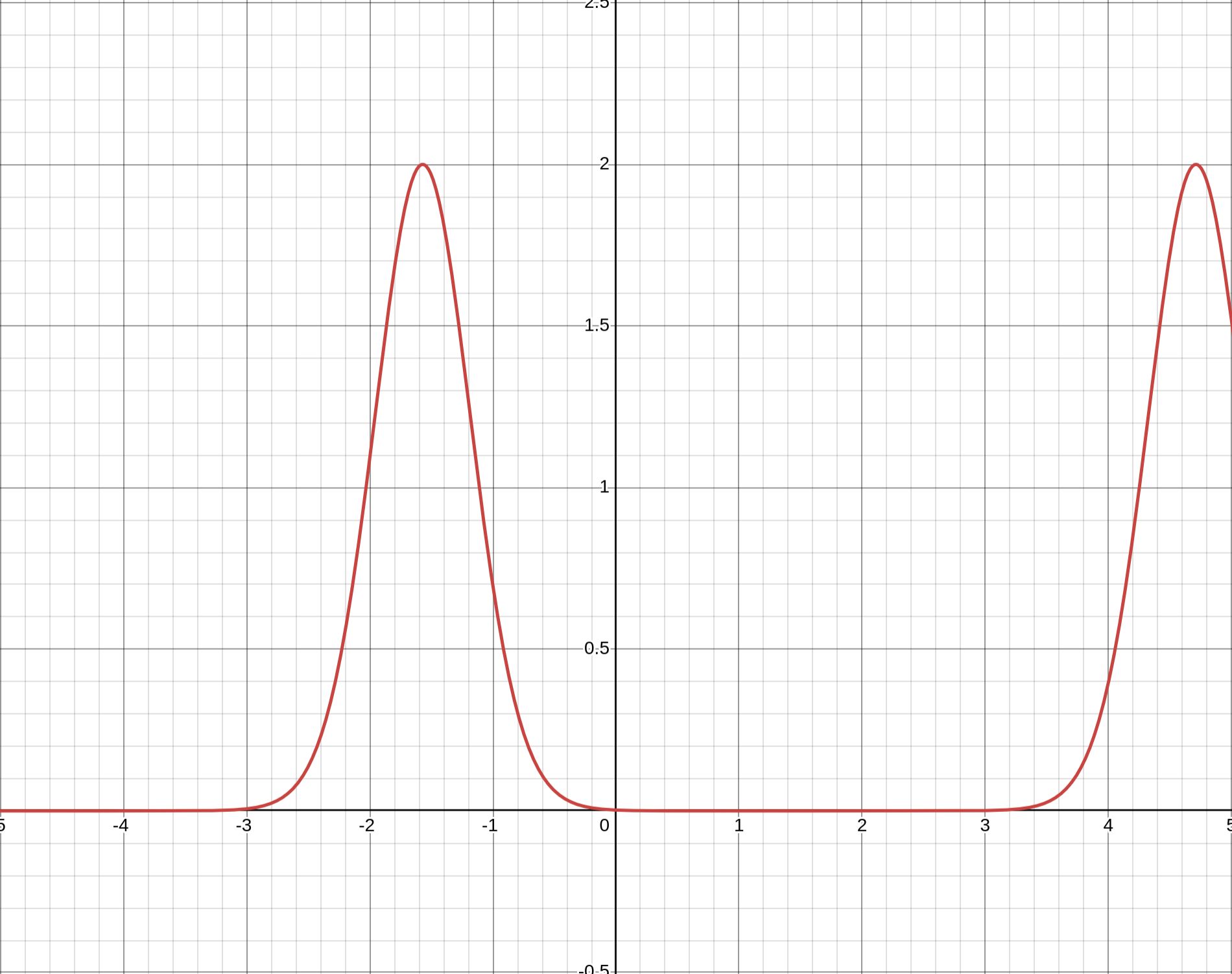
For this graph we set \(\delta=0.2\) and obtain a periodic result based on our input \(\theta\) on the \(x\)-axis. We see that there are many values of \(\theta\) for which \(\mathbb{P}(|X-\mu|\geq0.2\mu)\) is essentially 0. Funny stuff. Below is a graph for \(\delta=0.1\).
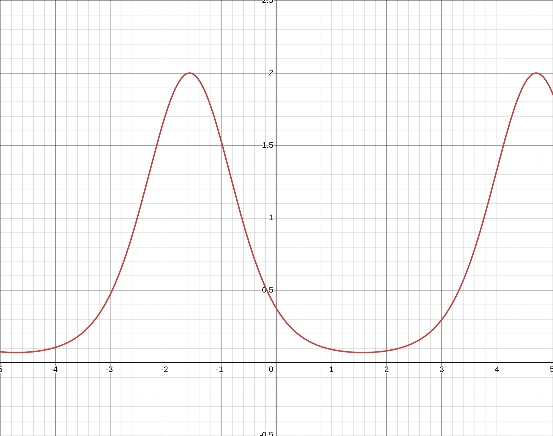
We can also use Chebyshev's Inequality to obtain the following bound given that our random variables are i.i.d., which thankfully they are:
$$ \mathbb{P}\left(\left|\frac{X}{n}-\mu\right|\geq\epsilon\right)\leq\frac{\sigma^2}{n\epsilon^2} $$
This bound is easier to understand from the formula than Chernoff. Plugging in our known values and taking \(\epsilon=\sqrt{1/120}\), we get \(\mathbb{P}(\left|\frac{X}{1000}-\mu\right|\geq 0.0913)\leq 0.01\). So there is at most a 1% chance that our output varies by more than 0.0913 when we compute over 1000 shots.
This was all not very important, but it was to say that the computation of the quantum layer does not have massive variance.
So is the whole story of the forward computation that it ultimately computes \(\frac{1+\sin(\theta)}{2}\) plus a small amount of variance? Yes. It actually could've been more complicated than that if the authors had used a noise model with the simulation, which would model more factors of quantum error, but they didn't.
So now you might say: okay so what that the quantum layer just computes \(\frac{1+\sin(\theta)}{2}\), that's still probably somewhat valuable right? I honestly don't think it is. Remember, there are no trainable parameters here; it is a constant transform. And given that the last fully-connected layer had no activation function after, we can basically treat this computation as an activation function - a sinusoidal activation function with noise.
If you explore the research on using sinusoidal activation functions, you will find that they are determined to be pretty difficult to train and not worth using due to their horrific local minima as a periodic function [1]. And if you explore the use of noise layers, they have sometimes been used to increase model robustness, however I believe it has been largely proven that dropout is far more effective.
Anyway, we still have to cover the backpropagation.
def backward(ctx, grad_output):
    x, = ctx.saved_tensors
    input_list = np.array(x.tolist())

    shift_right = input_list + np.ones(input_list.shape) * ctx.shift
    shift_left = input_list - np.ones(input_list.shape) * ctx.shift

    gradients = []
    for i in range(len(input_list)):
        expectation_right = ctx.quantum_circuit.run(shift_right[i])
        expectation_left = ctx.quantum_circuit.run(shift_left[i])

        gradient = torch.tensor([expectation_right]) - torch.tensor([expectation_left])
        gradients.append(gradient)
    gradients = np.array([gradients]).T
    return torch.tensor([gradients]).float() * grad_output.float(), None, None
ctx.shift is defined earlier in the forward() function. They didn't set the shift parameter to a non-default value in the QuantumHybridModel constructor, so it is always \(\pi/2\). This makes for a funny behavior. They seem to attempt to do some sort of finite difference method approach for approximating the gradient. They run the quantum circuit \(q\) on \(q(\mathbf{x}+\pi/2)\) and \(q(\mathbf{x}-\pi/2)\) and take their difference as the gradient. But remember, this means we have \(\frac{1+\sin(\theta+\pi/2)-1-\sin(\theta-\pi/2)}{2}=\frac{\cos(\theta)-(-\cos(\theta))}{2}=\cos(\theta)\), which is unfortunately double the correct gradient \(\frac{\cos(\theta)}{2}\).
And it gets worse. For whatever reason they also transpose the gradients, so once they're multiplied by the oncoming gradient output, we end up with a \(2\times 2\) matrix, which doesn't really make any sense. I've thought a lot about it and I genuinely can't make sense of what this would even mean.
So now you see what's so funny about this quantum layer business. The supposed benefit of representing fewer states with fewer model parameters isn't used at all; it's just a sine function! Is there memory saved? No. Is computational cost lower? Absolutely not, if anything it's much higher! The quantum circuit has to be simulated 1000 times every forward pass and 2000 more times every backward pass!
This concludes my issues with this project. I want to emphasize I'm not hating on the authors of this project at all though. Hackathons are great for learning new things and I'm sure they didn't realize they just implemented a sine function. I mostly just thought it was funny, though I am a bit upset with the judges of this category as there were other projects that implemented legitimate quantum algorithms like QAOA for real applications. These projects would actually have legitimate use in a world where quantum computers were available, whereas this really doesn't provide any valuable use of quantum computing.
In any case, it was a fun exploration to uncover the issues with the project.