Seeing the popularity of Frank Herbert's Dune in 2024, for UMDCTF we decided to make Dune our theme. But we were left with the question: how should we theme the challenge list to fit a Dune aesthetic? And I had the brilliant idea of making a 3D Dune planet visualization as the challenge interface. It didn't work out as planned, at least not fully...
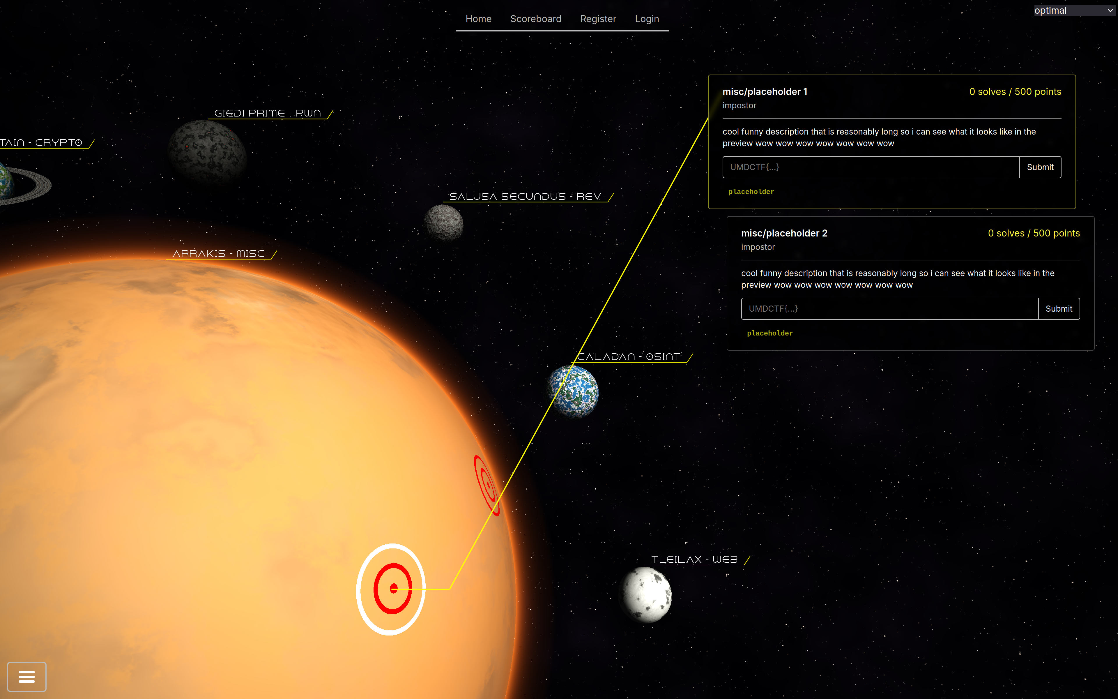
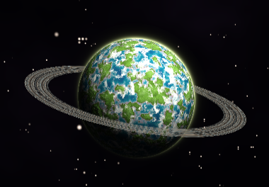
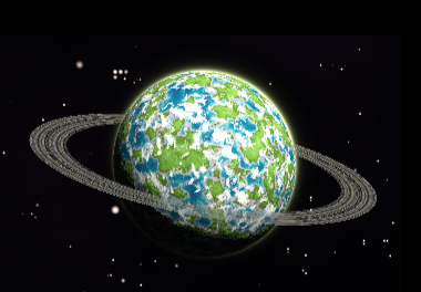
I've embedded the simulation above, along with some controls to mimic the challenge interface during the CTF. The actual interface looked cooler than this (I can't be bothered implementing the whole challenge list for this post), you can see below:
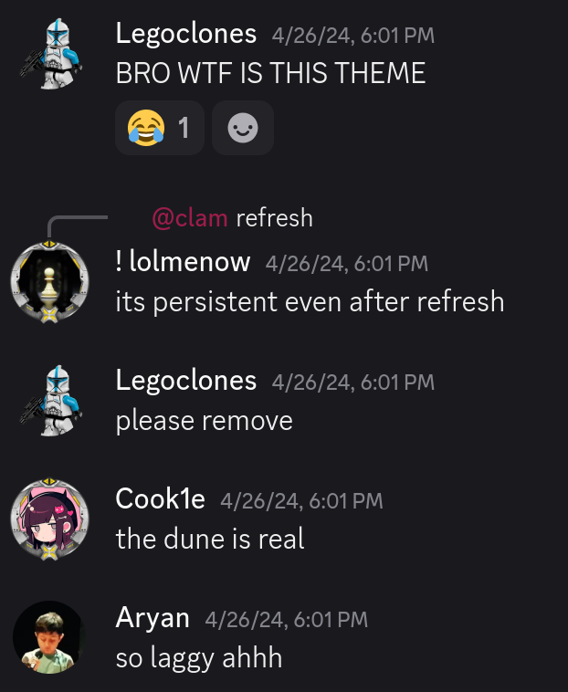
I spent a lot of time working on this, and it looks pretty cool in my opinion, so you could imagine I was excited for everyone to see it when the CTF started. Unfortunately, the reaction was not quite as positive as I anticipated:
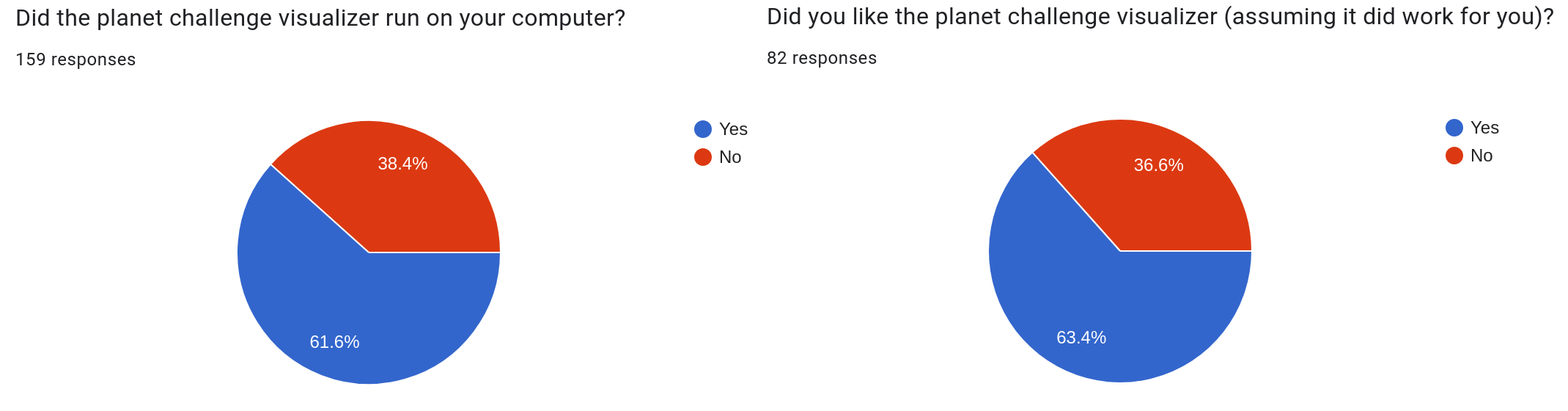
Yeah... There might have been performance issues. It also straight up did not run on some systems, and to this day I don't really understand why. We did a poll at the end of the CTF on whether it ran on peoples' systems and if they liked it:
So yeah, it wasn't the most successful endeavor. Still, there is a lot of technical depth to the simulation that I want to cover in this post because I think it's pretty cool.
I wrote the simulation using WebGL2, which is basically just OpenGL ES 3.0 for the web. You might wonder how many triangles I'm rendering to get such smooth spherical planets. The answer? 2.
That's right, this isn't rasterized at all, I'm just rendering two triangles for the screen surface. The entire thing is rendered using raycasting in the shader. The shader is heavily based on Julien Sulpis's realtime planet shader, and I'd like to use this post as an attempt to explain the machinations of such a shader.
A standard raycasting fragment shader is as follows:
in vec2 uv;
out vec4 fragColor;

uniform vec3 uCameraPosition;

void main() {
    vec3 ro = uCameraPosition;
    vec3 rd = normalize(vec3(uv, -1.));

    fragColor = vec4(radiance(ro, rd), 1.);
}
For those unfamiliar, a shader is essentially a program that executes on the GPU. A very basic shading pipeline will have a vertex shader and a fragment shader. The vertex shader will run for every vertex rendered (where there are of course 3 per triangle). And the fragment shader will run for every "fragment", which typically is just each pixel unless you're doing multisampling/antialiasing.
A vertex shader can optionally pass data to the fragment shader, which we are doing in this case with the uv parameter. The way this is calculated is fairly unimportant, but just know that UV coordinates are intended to be texture coordinates when rendering a primitive shape. In our case, our surface is a square and our UV coordinates are from \([-0.5, 0.5]\) on both the \(x\) and \(y\) axes.
Now, what are these ro and rd variables? ro is short for ray origin, or the point from which the ray we cast originates in world space. We set this to uCameraPosition, which is a uniform variable storing the current position of the camera in world space. And for those unfamiliar, a uniform is a shader variable whose value can be set from the CPU side of the renderer before the draw call.
rd is short for ray direction, or the direction in which we are casting the ray in world space. But what is this normalize(vec3(uv, -1.)) calculation doing?
If you imagine a camera taking a picture, this camera obviously has a position and it also has a direction it's facing. But now think from the perspective of the sensor in that camera. How does it capture an image? There are light rays bouncing around in the world, which eventually bounce into the sensor. This light is captured by the sensor at the exact point it hit, which then corresponds to the pixel in the captured image. That point on the sensor is essentially our UV coordinate. We intend to replicate this natural process but in reverse - we will shoot rays from the camera rather than capturing rays incoming to the camera. We intend to shoot one ray for each pixel in the image.
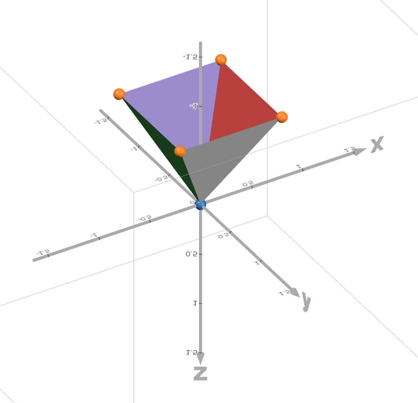
For our case, we don't need to vary camera direction so we just assume the camera faces in the negative \(z\) direction, which makes our computation of ray direction simple. We just use our UV coordinate as the \((x,y)\) components of our ray direction, with \(z=-1\). This forms a pyramid of possible ray directions given \(uv\in[-0.5,0.5]\times[-0.5,0.5]\), seen here:
All that's left to be explained is the radiance(ro, rd) function. Unsurprisingly, that's where the bulk of the computation comes in.
vec3 radiance(vec3 ro, vec3 rd) {
    vec3 color = vec3(0.);
    float spaceMask = 1.;
    Hit hit = intersectScene(ro, rd);
    Hit ringHit = intersectRing(ro, rd);

    if (hit.len < INFINITY) {
        spaceMask = 0.;

        vec3 hitPosition = ro + hit.len * rd;
        Hit shadowHit = intersectScene(hitPosition + EPSILON * SUN_DIRECTION, SUN_DIRECTION);
        float hitDirectLight = step(INFINITY, shadowHit.len);

        float directLightIntensity = pow(clamp(dot(hit.normal, SUN_DIRECTION), 0.0, 1.0), 2.) * SUN_INTENSITY;
        vec3 diffuseLight = hitDirectLight * directLightIntensity * SUN_COLOR;
        vec3 diffuseColor = hit.material.color.rgb * (AMBIENT_LIGHT + diffuseLight);

        vec3 reflected = normalize(reflect(SUN_DIRECTION, hit.normal));
        float phongValue = pow(max(0.0, dot(rd, reflected)), 10.) * .01 * SUN_INTENSITY;
        vec3 specularColor = hit.material.specular * vec3(phongValue);

        color = diffuseColor + specularColor;
    } else {
        color = spaceColor(rd);
    }

    if (ringHit.len < hit.len) {
        color = color * (1. - ringHit.material.color.a) + ringHit.material.color.rgb;
        spaceMask = 0.;
    }

    if (uHoveredPlanet != uSelectedPlanet) {
        color += atmosphereColor(uHoveredPlanet, ro, rd, spaceMask, hit, ringHit);
    }
    return color + atmosphereColor(uSelectedPlanet, ro, rd, spaceMask, hit, ringHit);
}
We start by testing if our ray intersects with the scene (planets and moons) and the planet Kaitain's ring (more on why this needs to be a separate check later). Don't worry about how these intersection tests work just yet, I'll get there later.
If we intersected the scene, that means we must've hit a planet or a moon. Our spaceMask variable is essentially a boolean on whether we hit empty space or not, and we didn't so we set this to 0. We calculate the position of the hit by rather intuitively multiplying our ray direction by the ray length (recall how we normalized ray direction) and adding the ray origin.
Now that we know where we hit, we can cast another ray from this point in the direction of the sun, which determines if there should be a shadow cast on our hit point. We only intersect with the scene and not the ring because we treat the ring as translucent for simplicity. We then use the builtin GLSL step() function to calculate hitDirectLight, a boolean representing if we hit direct light or not (0 if we hit an object on the shadow cast and 1 if not).
From here we can determine the color of the pixel resulting from our ray hit. We will be using the Phong reflection model for this.
We first attempt to determine the intensity of the light from the sun. According to Lambert's cosine law, when a light ray hits a diffuse (think: matte) surface, the intensity of the diffuse light is proportional to the cosine of the angle between the surface normal (the perpendicular direction at the point hit on the surface) and the direction of the incoming light. If you have two normalized vectors, then their dot product is the cosine of the angle between them. We then clamp that value in \([0,1]\) to avoid any pesky edge cases where somehow the angle is greater than \(90\degree\). And finally we take this cosine and square it, which is technically not physically accurate but it creates a slightly softer shadow curve which I think looks nice. See below, the first squared and second realistic.
And we also multiply by some constant sun intensity value, which we define as 3. We now have the intensity of direct light from the sun. To obtain our actual diffuse light radiance, we simply multiply this by our direct light boolean and a constant sun color vector (defined as vec3(1.0, 1.0, 0.9), a pale yellow). We then take this value, add a constant ambient light in the scene, and multiply by our surface color at the point hit. We finally have computed diffuse radiance.
Now we need specular (shiny, reflective) radiance. According to the Phong model, specular radiance is proportional to some power of the cosine of the angle between the path from the surface to the viewer and the direction of a reflected light ray. Put mathematically:
$$ I_s=k_s(R\cdot V)^\alpha i_s $$
With \(R,V\) given as the vectors in this image:
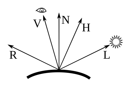
Thus we compute the reflected direction of a sun ray off of our surface, take the dot product of this with our ray direction, and take it to the power of \(\alpha=10\). This power corresponds to how shiny the surface is, with a higher power resulting in a smaller, brighter highlight. We then multiply by 0.01 * SUN_INTENSITY to reduce the significance of specular highlights. This is essentially our \(k_s\). And finally we multiply by the surface's specular color component at the hit point, our \(i_s\).
And finally our color for this hit is just the sum of the diffuse and specular components. Whew, that was a lot. And in the case where we don't hit a planet or moon, our color is just the color of space (we'll see this in a bit).
To provide some idea of what this Phong model actually does, here is a solid red planet without all the fancy terrain coloring and clouds:
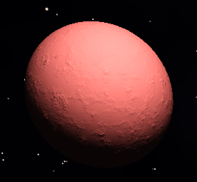
We get a subtle highlight in the top right where the sunlight is coming from. The planet gets darker as we get further from the sun. And the roughness of the surface comes from our computed planet normals not being perfectly smooth, but rather attempting to simulate a rough planet surface with mountains (which we will see later).
Now this next part is why we need the ring hit to be processed separately from the scene. We want to blend between the color of the ring and the color behind the ring to make the ring translucent. So if we hit a ring and the ring hit ray distance is less than that of the scene (the ring is in front of the planet/moon/space), then we compute our color as the ring color plus the previously computed color scaled down by one minus the transparency of the ring. I found this yielded a nice translucent-like appearance.
We're almost done with this function. You may have noticed that we treat the atmosphere as a hover indicator for non-selected planets. We simply add the atmosphere color to our total color if we are hovering over a planet. And we also always render the atmosphere for the selected planet, so we add that too. That's it!
But we have a long way to go. How does the scene intersection work? How does the ring intersection work? How is the space color calculated? What about the atmosphere color? Let's start with atmosphere color because I think it's simplest.
vec3 atmosphereColor(int planetIndex, vec3 ro, vec3 rd, float spaceMask, Hit firstHit, Hit ringHit) {
    vec3 position = ro + firstHit.len * rd;

    Planet planet = planets[planetIndex];
    vec3 planetPosition = uPlanetPositions[planetIndex];

    float distCameraToPlanetOrigin = length(planetPosition - ro);
    float distCameraToPlanetEdge = sqrt(distCameraToPlanetOrigin * distCameraToPlanetOrigin - planet.radius * planet.radius);

    float satelliteMask = smoothstep(-planet.radius / 2., planet.radius / 2., distCameraToPlanetEdge - firstHit.len);
    float ringMask = step(ringHit.len, distCameraToPlanetEdge) * ringHit.material.color.a;
    float planetMask = 1.0 - spaceMask;

    vec3 coordFromCenter = (ro + rd * distCameraToPlanetEdge) - planetPosition;
    float distFromEdge = abs(length(coordFromCenter) - planet.radius);
    float planetEdge = max(planet.radius - distFromEdge, 0.) / planet.radius;
    float atmosphereMask = pow(remap(dot(SUN_DIRECTION, coordFromCenter), -planet.radius, planet.radius / 2., 0., 1.), 3.);
    atmosphereMask *= planet.atmosphereDensity * planet.radius * SUN_INTENSITY;

    vec3 planetAtmosphere = vec3(0.);
    planetAtmosphere += vec3(pow(planetEdge, 120.)) * .5;
    planetAtmosphere += pow(planetEdge, 50.) * .3 * (1.5 - planetMask);
    planetAtmosphere += pow(planetEdge, 15.) * .03;
    planetAtmosphere += pow(planetEdge, 5.) * .04 * planetMask;
    planetAtmosphere *= planet.atmosphereColor * atmosphereMask * (1.0 - planetMask * min(satelliteMask + ringMask, 1.))  * step(distFromEdge, planet.radius / 4.);
    return planetAtmosphere;
}
The core idea of this function is that we want to create an atmosphere that smoothly fades as you exit the radius of the planet edge. Using the Pythagorean theorem, we can obtain the distance from the camera to the edge of the planet. Of course, there are infinitely many edges I could be referring to, but since this is the Pythagorean theorem, this applies to right triangles, so this is the edge perpendicular to the vector from the camera to the planet origin. See the below visualization:
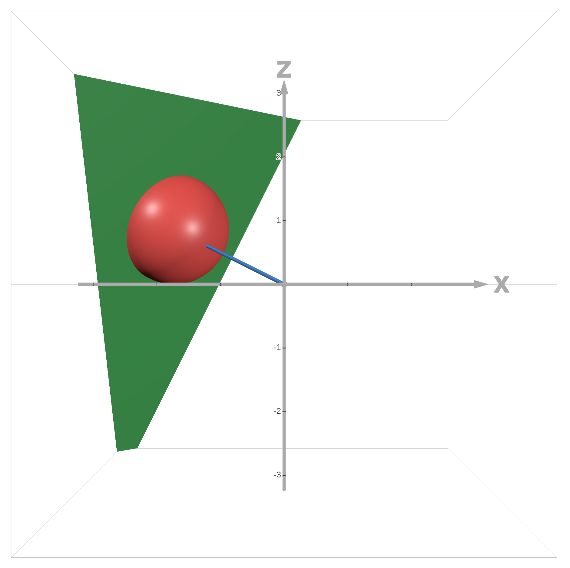
The relevant edges are the edges at the intersection of the sphere and the plane.
We then use this distance to calculate what we call a satellite mask. We use the smoothstep() function to smoothly interpolate between 0 and 1 for a value between two edge values. If distCameraToPlanetEdge - firstHit.len < -planet.radius / 2 then we get 0, if distCameraToPlanetEdge - firstHit.len > planet.radius / 2 we get 1, and in between we get a smooth interpolation. The purpose of this satellite mask is to ensure we don't draw the atmosphere over an orbiting body in front of the atmosphere. Imagine we have a moon on the right edge of our planet in front. The firstHit.len will be less than the distCameraToPlanetEdge, so we will approach 1 for the satellite mask. Now let's say the moon is on the right edge but behind the planet. Then the firstHit.len will be much longer than distCameraToPlanetEdge, so the satellite mask will be 0. This is exactly what we want, and we will use it later to ensure the atmosphere is drawn over the satellite when the satellite is behind the planet, but not in front. And because we use smoothstep() we get a smooth transition between the two states as the satellite orbits.
We now also compute a ring mask for the same reason, but also include the ring transparency as a factor because we want the ring to be somewhat translucent. And of course, we don't want to draw the atmosphere on the body of the planet, so we compute a planet mask as well using our previously computed space mask.
Now we attempt to find a reasonable approximation for the distance from our ray to the edge of the planet. We want the atmosphere to be strongest right at the edge and fade as we get farther from the edge. In many cases when the ray is near the edge but not hitting the planet, the ray will not actually be hitting anything, so we need some distance to use that gets us close to the planet edge. Well good thing we have distCameraToPlanetEdge. We use this to get a point on our ray close to the planet edge, and then we subtract the planet position to get a vector from the center of the planet to our point. We then compute the distance from this point to the edge of the planet. But we're not done. We want to obtain a value in \([0,1]\) representing our atmosphere strength due to the distance. So we subtract the distance from the edge from the planet radius, clamping the minimum value to 0, and then dividing by the planet radius. This gives a value of 1 at the planet edge, falling off to 0 at a planet radius away from the edge.
Now we want to get that cool atmospheric effect where it appears stronger in the direction of the sun. We once again use our dot product with the sun direction trick, but now we remap this value from the range of \([-r,r/2]\) to \([0,1]\), with \(r\) our planet radius. This gives a smooth transition from the opposite side of the planet from the sun having no atmosphere to the side directly facing the sun having full atmosphere. And to get a more dynamic nonlinear curve, we take this to the power of 3. And finally we multiply this by our planet's atmospheric density, and then further scale it by the planet's radius and the sun intensity.
We're almost done. The next several lines are essentially trying to build an interesting atmospheric falloff curve by taking powers of the planetEdge value (remember it's in \([0,1]\)) and giving them some scale and adding them together. The numbers are very arbitrary but yield a nice result.
Our final step is combining everything together. We multiply our dynamic falloff curve by the atmosphere color and the sun strength effect mask. We then multiply by 1.0 - planetMask * min(satelliteMask + ringMask, 1.), which is equivalent to saying we don't want to draw the atmosphere wherever planetMask is 1 and satelliteMask or ringMask is 1. This ensures we don't draw over satellites and rings in front of the planet. And finally we cut the atmosphere off at a distance of a fourth the radius from the edge.
So now we know how the atmosphere is determined. I think the next logical step is talk about the space color.
vec3 spaceColor(vec3 direction) {
    vec3 backgroundCoord = direction;
    float spaceNoise = fbm(backgroundCoord * 3., 4, .5, 2., 6.);

    return stars(backgroundCoord) + mix(DEEP_SPACE, SPACE_HIGHLIGHT / 12., spaceNoise);
}
Super simple right? Well, maybe if you already know what fractal Brownian motion is. Rather than attempt to explain fBm in great detail, I will link a relevant chapter of The Book of Shaders. For a brief summary, it's essentially a noise function that yields self-similar noise patterns, which are often used in graphics for things like procedural landscapes. In this particular call, we use 4 octaves, 0.5 persistence, 2 lacunarity, and 6 exponentiation.
And by the way, I'm not even going to attempt to explain the stars() function. It's one of those pieces of Shadertoy magic that you always seem to encounter when you're into shader programming. It originates from this shader by nimitz.
Anyways, the space color is just the magic stars plus a linear interpolation between the color of deep space and a space highlight color based on the fBm noise.
Alright, onto ring intersection.
Hit intersectRing(vec3 ro, vec3 rd) {
    vec3 planeParam = normalize(vec3(0.2, 1., 0.5));
    vec3 kaitainPosition = uPlanetPositions[5];
    float len = plaIntersect(ro, rd, vec4(planeParam, -dot(planeParam, kaitainPosition)));
    if (len < 0.) {
        return miss;
    }

    vec3 position = ro + len * rd;
    float l = length(position.xz - kaitainPosition.xz);

    if (l > 7.5 && l < 9.5) {
        float density = 1.2 * clamp(noise(vec3(l * 20.)), 0., 1.) - .2;
        vec3 color = mix(vec3(.42, .3, .2), vec3(.41, .51, .52), abs(noise(vec3(l * 19.)))) * abs(density);
        return Hit(len, planeParam, Material(vec4(color, density), 1., 0.));
    }
    return miss;
}
We define a plane that the ring sits in. planeParam is the normal vector defining the plane. We have a plaIntersect() function which determines ray intersection with a plane. In order to define the plane for this function, we need a 4 values corresponding to \(a,b,c,d\) in the plane equation \(ax+by+cz+d=0\). \((a,b,c)\) defines our normal vector, so we just need to choose \(d\) so the plane passes through the planet position. This is satisfied precisely when \(d\) is the negative dot product of the plane normal vector and the planet position.
The plaIntersect() function comes from Inigo Quilez's article on ray-surface intersectors. For those unaware, he is one of the goats of computer graphics.
After computing the plane intersection, if the ray length is negative that means we missed. Otherwise we compute the ray hit position and use it to compute a radius to the center of the planet in the \(xz\)-plane. We then draw the ring in the \(xz\) radius \([7.5,9.5]\). In order to get a concentric noise pattern for our ring density, we sample noise using our radius, which we scale up to increase the frequency of the noise. We scale up this result by 1.2 and subtract 0.2 to keep it at most 1 but vary the result. We then determine the color by linearly interpolating between two colors of our choosing based on another noise sample using our radius. We then multiply this by the absolute value of our computed density, which yields the overall color of the ring. We also use this density as the transparency term of the ring. Not too complicated.
Now finally onto the scene intersection.
Hit intersectScene(vec3 ro, vec3 rd) {
    for (int i = 0; i < 6; i++) {
        Hit hit = intersectPlanet(i, ro, rd);
        if (i == uSelectedPlanet) {
            Hit moonHit = intersectMoon(i, ro, rd);

            if (moonHit.len < hit.len) {
                return moonHit;
            }
        }

        if (hit.len < INFINITY) {
            return hit;
        }
    }

    return miss;
}
It's pretty straightforward. We iterate over our planets, intersect them, and for the selected planet we also intersect the moon and return whichever hit is closer. Moon intersection is as follows:
Hit intersectMoon(int planetIndex, vec3 ro, vec3 rd) {
    Hit hit = miss;
    Planet planet = planets[planetIndex];
    vec3 planetPosition = uPlanetPositions[planetIndex];
    for (int i = 0; i < planet.moonCount; i++) {
        Moon moon = planet.moons[i];
        vec3 moonPosition = currentMoonPosition(planetIndex, i);
        float len = sphIntersect(ro, rd, moonPosition, moon.radius);

        if (len < 0.) {
            continue;
        }

        vec3 position = ro + len * rd;
        vec3 originalPosition = (position - planetPosition) * rotate3d(moonRotationAxis(planetIndex, i), -uTime * moon.rotationSpeed);
        vec3 color = vec3(sqrt(fbm(originalPosition * 12., 6, .5, 2., 5.)));
        vec3 normal = normalize(position - moonPosition);

        if (len < hit.len) {
            hit = Hit(len, normal, Material(vec4(color, 1.), 1., 0.));
        }
    }

    return hit;
}
For each moon of the given planet, we compute the current moon position by rotating it about the moon's rotation axis by the current time times the moon's rotation speed. We then do a sphere intersection to see if we hit the moon. If we do, we determine the hit position and use it to determine the moon's original position at the beginning of the simulation before it began orbiting the planet. We use this to obtain a consistent noise pattern for the color of the moon, because otherwise the noise would change as it orbits around the planet. We sample fBm noise, take the square root to make it more gray, and use the result as grayscale color. We then compute smooth spherical normals, and update our returned hit if this hit is the shortest of all the moons (i.e. it is in front).
Then all that's left is the planet intersection, which is perhaps the most interesting part of all.
Hit intersectPlanet(int planetIndex, vec3 ro, vec3 rd) {
    Planet planet = planets[planetIndex];
    vec3 planetPosition = uPlanetPositions[planetIndex];
    float len = sphIntersect(ro, rd, planetPosition, planet.radius);

    if (len < 0.) {
        return miss;
    }

    vec3 position = ro + len * rd;
    vec2 rotationAmt = vec2(uTime * ROTATION_SPEED / planet.radius, 0.) + step(float(planetIndex), float(uSelectedPlanet)) * step(float(uSelectedPlanet), float(planetIndex)) * uRotationOffset;
    vec3 rotatedCoord = rotate3d(rotateY(PI / 5. + rotationAmt.x) * vec3(0, 0, -1), rotationAmt.y) * rotateY(rotationAmt.x) * (position - planetPosition);
    float altitude = 5. * planetNoise(planet, rotatedCoord);

    vec3 normal = planetNormal(planetIndex, position);

    vec3 color = mix(planet.waterColorDeep, planet.waterColorSurface, smoothstep(planet.waterSurfaceLevel, planet.waterSurfaceLevel + planet.transition, altitude));
    color = mix(color, planet.sandColor, smoothstep(planet.sandLevel, planet.sandLevel + planet.transition / 2., altitude));
    color = mix(color, planet.treeColor * min(((altitude - planet.treeLevel) / (planet.rockLevel - planet.treeLevel) + .3), 1.), smoothstep(planet.treeLevel, planet.treeLevel + planet.transition, altitude));
    color = mix(color, planet.rockColor, smoothstep(planet.rockLevel, planet.rockLevel + planet.transition, altitude));
    color = mix(color, planet.iceColor, smoothstep(planet.iceLevel, planet.iceLevel + planet.transition, altitude));

    vec3 cloudsCoord = (rotatedCoord + vec3(uTime * .008 * planet.cloudsSpeed)) * planet.cloudsScale;
    float cloudsDensity = remap(domainWarpingFBM(cloudsCoord, 3, .3, 5., planet.cloudsScale), -1.0, 1.0, 0.0, 1.0);
    float cloudsThreshold = 1. - planet.cloudsDensity * .5;
    cloudsDensity *= smoothstep(cloudsThreshold, cloudsThreshold + .1, cloudsDensity);
    cloudsDensity *= smoothstep(planet.rockLevel, (planet.rockLevel + planet.treeLevel) / 2., altitude);
    color = mix(color, planet.cloudColor, cloudsDensity);

    if (planetIndex == uSelectedPlanet) {
        for (int j = 0; j < uChallengeCount; j++) {
            float d = distance(challengePoints[j] * planet.radius, rotatedCoord) / planet.radius;
            color = mix(color, vec3(1.) - vec3(0., 1., 1.) * (sin(uTime * 5.) + 4.) / 2., step(d, .01));
            color = mix(color, vec3(1.) - vec3(0., 1., 1.) * (sin(uTime * 5. + 1.) + 4.) / 2., min(1., step(d, .05) * step(.04, d) + step(d, .09) * step(.08, d)));
            color = mix(color, vec3(1.) - vec3(0., 1., 1.) * (sin(uTime * 5. + 2.) + 4.) / 2., min(1., step(d, .09) * step(.08, d)));
        }
    }

    float specular = smoothstep(planet.sandLevel + planet.transition, planet.sandLevel, altitude);

    return Hit(len, normal, Material(vec4(color, 1.), 1., specular));
}
We start with the standard sphere intersection and computation of the hit position. We then determine the amount the planet has rotated. The standard rotation about the vertical axis is just the current time times the rotation speed scaled down by the planet's radius. But we also need to account for the uRotationOffset uniform, which we use to rotate the planet when selecting a challenge. But we only want to include this factor if the planet is selected, so we multiply by two step functions which avoids an if statement, making this branchless (meaning there are no branch conditions that would cause multiple executions to diverge in execution), which is desirable in shaders because GPUs are highly parallel and benefit from consistent execution across threads.
We then use the rotation amount to rotate the vector from the planet origin to our hit point. This gives us a coordinate on the planet surface. We use this to sample our planet noise, which is essentially just an fBm sample that also flattens the noise out in the ocean areas. We use the returned value as our altitude at the given coordinate.
We proceed to call planetNormal(), which uses the finite difference method to compute the normal at the hit position, accounting for the planet noise for terrain.
Once we've done all that, we can start getting into the colors of the terrain. The determination of the color uses a series of linear interpolations between different altitude levels, which are defined per planet. We start out by blending between the deep water color and the shallow water color based on where our altitude falls in the range from the water surface level and the water surface level plus some transition value. We proceed to chain very similar operations with all the different terrain types and we ultimately get the right color corresponding to our altitude.
Now onto clouds. We compute a cloud coordinate using our rotated planet coordinate, adding a factor for cloud movement. To compute cloud density, we use a domain warping fBm sample remapped from \([-1,1]\) to \([0,1]\). Domain warping was mentioned in the Book of Shaders chapter I linked earlier, but for more information also reference Inigo Quilez's article on the subject. The brief summary is that we use fBm noise to warp fBm noise, which can yield a cloud-like movement effect. We then calculate cloudsThreshold and multiply our density by a smoothstep of the threshold to create a smooth falloff for the density. We also include a factor of altitude interpolation to ensure our altitude is at least above rock and tree level when clouds are showing. Finally, we interpolate between our previously calculated color and the cloud color based on our computed cloud density.
We only have a couple steps left. If this planet is our selected planet, we also want to draw the indicators on the surface for our challenges. For each challenge, we compute a distance from the challenge point on the surface to the rotated coord, of course scaled down by the planet's radius. This value acts as a radius on the surface, allowing us to render circular shapes on the planet's surface. I intended to use this series of linear interpolations to create a red and white flashing bullseye, but somehow I made a mistake somewhere that resulted in weird yellow artifacts appearing. Now that I'm looking at it again, I see the bug, but I'll leave it as an exercise for the reader to determine. Anyways, I actually really liked the yellow bug, a lot more than the plain red and white that I intended, so I didn't bother figuring it out and just left it. I think it adds character.
Finally, we compute the specular component by smoothly interpolating between 1 at or below the sand altitude level and 0 at or above the sand altitude level plus our planet's altitude transition value.
That's it! We've pretty much covered the entire planet shader! If you want to see the source, your browser probably already requested it to run the simulation at the top of the page. Here's the link. And the WebGL source is in a script tag in the page source as well.